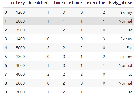
1. 데이터 생성
import pandas as pd
df = pd.DataFrame(columns=['calory', 'breakfast', 'lunch', 'dinner', 'exercise', 'body_shape'])
df.loc[0] = [1200, 1, 0, 0, 2, 'Skinny']
df.loc[1] = [2800, 1, 1, 1, 1, 'Normal']
df.loc[2] = [3500, 2, 2, 1, 0, 'Fat']
df.loc[3] = [1400, 0, 1, 0, 3, 'Skinny']
df.loc[4] = [5000, 2, 2, 2, 0, 'Fat']
df.loc[5] = [1300, 0, 0, 1, 2, 'Skinny']
df.loc[6] = [3000, 1, 0, 1, 1, 'Normal']
df.loc[7] = [4000, 2, 2, 2, 0, 'Fat']
df.loc[8] = [2600, 0, 2, 0, 0, 'Normal']
df.loc[9] = [3000, 1, 2, 1, 1, 'Fat']
df.head(10)
[출력]
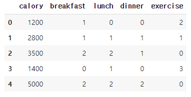
2. 데이터 전처리
데이터 특징으로만 구성된 X 데이터프레임 생성
X = df[['calory', 'breakfast', 'lunch', 'dinner', 'exercise']]
X.head()
[출력]
3. 표준화
모든 특성들을 평균이 0이고 표준편차가 1인 데이터로 바꾼 후 비교하면 특성들의 상관관계를 이해하기가 쉬워지고 효율적으로 학습할 수 있기 때문에 표준화를 해야한다.
from sklearn.preprocessing import StandardScaler
x_std = StandardScaler().fit_transform(X)
print(x_std)
[출력]
[[-1.35205803 0. -1.3764944 -1.28571429 1. ]
[ 0.01711466 0. -0.22941573 0.14285714 0. ]
[ 0.61612771 1.29099445 0.91766294 0.14285714 -1. ]
[-1.18091145 -1.29099445 -0.22941573 -1.28571429 2. ]
[ 1.89972711 1.29099445 0.91766294 1.57142857 -1. ]
[-1.26648474 -1.29099445 -1.3764944 0.14285714 1. ]
[ 0.18826125 0. -1.3764944 0.14285714 0. ]
[ 1.04399418 1.29099445 0.91766294 1.57142857 -1. ]
[-0.15403193 -1.29099445 0.91766294 -1.28571429 -1. ]
[ 0.18826125 0. 0.91766294 0.14285714 0. ]]
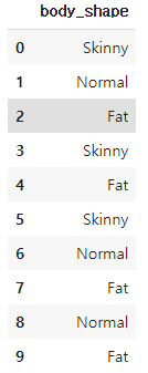
4. 레이블 분리
특성에 따른 레이블을 따로 데이터프레임으로 생성
Y = df[['body_shape']]
Y.head(10)
[출력]
5. 공분산 행렬 구하기
다음과 같이 np.cov로 공분산 행렬을 구할 수 있다.
import numpy as np
features = x_std.T #역행렬 (5*10)
covariance_matrix = np.cov(features) #covariance matrix
print(covariance_matrix)
[출력]
[[ 1.11111111 0.88379717 0.76782385 0.89376551 -0.93179808]
[ 0.88379717 1.11111111 0.49362406 0.81967902 -0.71721914]
[ 0.76782385 0.49362406 1.11111111 0.40056715 -0.76471911]
[ 0.89376551 0.81967902 0.40056715 1.11111111 -0.63492063]
[-0.93179808 -0.71721914 -0.76471911 -0.63492063 1.11111111]]
6. 고윳값과 고유벡터 구하기
np.linalg.eig로 고윳값(eigen value)와 고유벡터(eigen vector)를 구할 수 있다.
eig_vals, eig_vecs = np.linalg.eig(covariance_matrix)
print('Eigenvectors \n%s' %eig_vecs)
print('Eigenvalues \n%s' %eig_vals)
[출력]
Eigenvectors
[[-0.508005 -0.0169937 -0.84711404 0.11637853 0.10244985]
[-0.44660335 -0.36890361 0.12808055 -0.63112016 -0.49973822]
[-0.38377913 0.70804084 0.20681005 -0.40305226 0.38232213]
[-0.42845209 -0.53194699 0.3694462 0.22228235 0.58954327]
[ 0.46002038 -0.2816592 -0.29450345 -0.61341895 0.49601841]]
Eigenvalues
[4.0657343 0.8387565 0.07629538 0.27758568 0.2971837 ]
다음과 같이 계산하여 가장 큰 고유벡터로 데이터를 사영할 경우 얼마만큼의 정보가 유지되는지 확인 할 수 있다.
max(eig_vals) / sum(eig_vals)[출력]
0.7318321731427545
원본 데이터의 73% 정도에 해당하는 정보를 유지할 수 있다는 사실을 알 수 있다.
7. 5차원 데이터를 고유벡터로 사영
A벡터를 B벡터로 사영할 때의 공식은 dot(A, B) / Magnitude(B)이다.
#dot(A, B) / Magnitude(B)
projected_X = x_std.dot(eig_vecs.T[0]) / np.linalg.norm(eig_vecs.T[0])
projected_X
[출력]
array([ 2.22600943, 0.0181432 , -1.76296611, 2.73542407, -3.02711544,
2.14702579, 0.37142473, -2.59239883, 0.39347815, -0.50902498])
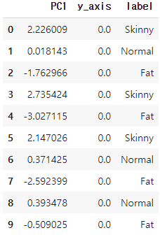
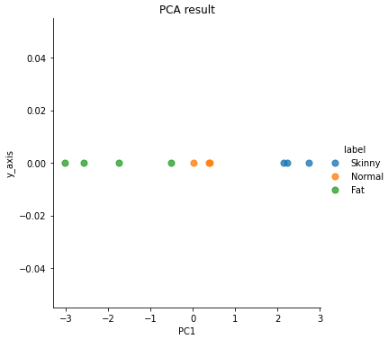
8. 시각화
result = pd.DataFrame(projected_X, columns=['PC1'])
result['y_axis'] = 0.0
result['label'] = Y
result.head(10)
[출력]
import matplotlib.pyplot as plt
import seaborn as sns
sns.lmplot('PC1', 'y_axis', data=result, fit_reg=False, scatter_kws={"s":50}, hue="label")
plt.title('PCA result')
[출력]
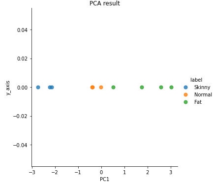
사이킷런을 활용한 주성분 분석
사이킷런 라이브러리를 쓰면 간단하게 주성분 분석을 구현할 수 있다.
from sklearn import decomposition
pca = decomposition.PCA(n_components=1) #PCA 모델 생성
sklearn_pca_x = pca.fit_transform(x_std) #모델 학습

sklearn_result = pd.DataFrame(sklearn_pca_x, columns=['PC1'])
sklearn_result['y_axis'] = 0.0
sklearn_result['label'] = Y
sns.lmplot('PC1', 'y_axis', data=sklearn_result, fit_reg=False, scatter_kws={"s":50}, hue="label")
plt.title('PCA result')
[출력]
'Machine Learning > Coding' 카테고리의 다른 글
| [실습] 단일, 다중 입력 로지스틱 회귀와 소프트맥스(다중 분류 로지스틱 회귀) (0) | 2021.07.12 |
|---|---|
| [실습] Linear Regression(선형회귀) (0) | 2021.06.27 |
| [실습] KMeans (K 평균 군집화) (0) | 2021.06.23 |
| [실습] 랜덤 포레스트(Random Forest)와 앙상블(Ensemble) (0) | 2021.06.20 |
| [실습] 다항분포 나이브 베이즈(Multinomial Naive Bayes) (0) | 2021.06.13 |