단일 입력 로지스틱 회귀
1. Import
from keras.models import Sequential
from keras.layers import Dense, Activation
import numpy as np
2. 모델 생성
#sigmoid(wx+b)의 형태를 갖는 간단한 로지스틱 회귀 구현
model = Sequential()
model.add(Dense(input_dim=1, units=1)) # 입력 1개, 출력 1개
model.add(Activation('sigmoid')) # 출력값을 시그모이드에 연결
model.compile(loss='binary_crossentropy',
              optimizer='sgd', metrics=['binary_accuracy'])
3. 데이터 생성
X = np.array([-2, -1.5, -1, 1.25, 1.62, 2])
Y = np.array([0, 0, 0, 1, 1, 1])
4. 모델 학습
model.fit(X, Y, epochs=300, verbose=0)5. 모델 예측
model.predict([-2, -1.5, -1, 1.25, 1.62, 2])[출력]
array([[0.13139299],
[0.19485846],
[0.27912793],
[0.7624209 ],
[0.8196183 ],
[0.8665657 ]], dtype=float32)
model.predict([-1000, 1000])[출력]
array([[0.],
[1.]], dtype=float32)
6. 모델 요약
단일 입력 로지스틱 모델은 한 개의 w와 b가 첫 번째 레이어에 존재한다. 학습 과정을 통해 최적의 w와 bias가 지정되고 dense 레이어에 2개의 param이 있는 것을 확인할 수 있으며 이 2개의 param이 w와 b이다. dense 레이어가 바로 선형 회귀 레이어인데 출력값은 activation 레이어의 입력으로 들어간다.
model.summary()[출력]

# 첫 번째 레이어에 존재하는 w와 b
model.layers[0].weights
[출력]
[<tf.Variable 'dense/kernel:0' shape=(1, 1) dtype=float32, numpy=array([[0.93990654]], dtype=float32)>,
<tf.Variable 'dense/bias:0' shape=(1,) dtype=float32, numpy=array([-0.0088849], dtype=float32)>]
 #학습을 통해 구한 최적의 w와 b
model.layers[0].get_weights()
[array([[0.93990654]], dtype=float32), array([-0.0088849], dtype=float32)]
다중 입력 로지스틱 회귀
1. Import
from keras.models import Sequential
from keras.layers import Dense, Activation
import numpy as np
2. 모델 생성
#sigmoid(w1x1 + w2x2 + b)의 형태를 띠는 로지스틱 회귀 구현
model = Sequential()
model.add(Dense(input_dim=2, units=1)) #입력 2개, 출력 1개
model.add(Activation('sigmoid'))
model.compile(loss='binary_crossentropy', optimizer='sgd', metrics=['binary_accuracy']) #크로스 엔트로피 비용함수와 경사하강법 사용
3. 데이터 생성
X = np.array([(0, 0), (0, 1), (1, 0), (1, 1)])
Y = np.array([0, 0, 0, 1])
4. 모델 학습
model.fit(X, Y, epochs=5000, verbose=0)5. 모델 예측
model.predict(X)[출력]
array([[0.5 ],
[0.37840027],
[0.5704581 ],
[0.44704354]], dtype=float32)
6. 모델 요약
다중 입력 로지스틱 모델은 w1, w2, b가 첫 번째 레이어에 존재하며 학습 과정을 통해 최적의 w1, w2, b가 지정된다. 아래에서 dense 레이어에 3개의 param이 존재하는 것을 확인할 수 있으며 이 3개의 param이 w1, w2, b이다. 또한 dense 레이어는 선형 회귀 레이어라고 볼 수 있으며 선형 회귀 레이어의 출력은 activation 레이어의 입력이 된다.
model.summary()[출력]

# 첫 번째 레이어에 존재하는 w1, w2, b
model.layers[0].weights
[출력]
[<tf.Variable 'dense/kernel:0' shape=(2, 1) dtype=float32, numpy=
array([[ 0.2837205 ],
[-0.49634385]], dtype=float32)>,
<tf.Variable 'dense/bias:0' shape=(1,) dtype=float32, numpy=array([0.], dtype=float32)>]
 # 최적의 w1, w2, b
model.layers[0].get_weights()
[출력]
[array([[ 0.2837205 ],
[-0.49634385]], dtype=float32), array([0.], dtype=float32)]
소프트맥스(다중 분류 로지스틱 회귀)
1. Import
from keras.models import Sequential
from keras.layers import Dense, Activation
from tensorflow.keras.utils import to_categorical
from keras.datasets import mnist
2. 데이터 획득
학습 데이터 하나를 출력해보면 각 픽셀이 0부터 255까지의 값을 가지고 있는 것을 확인 할 수 있다.
(X_train, y_train), (X_test, y_test) = mnist.load_data()
print("train data (count, row, column) :", str(X_train.shape))
print("test data (count, row, column) :", str(X_test.shape))
print(X_train[0])
[출력]
train data (count, row, column) : (60000, 28, 28)
test data (count, row, column) : (10000, 28, 28)[[ 0 0 0 0 0 0 0 0 0 0 0 0 0 0 0 0 0 0
0 0 0 0 0 0 0 0 0 0]
[ 0 0 0 0 0 0 0 0 0 0 0 0 0 0 0 0 0 0
0 0 0 0 0 0 0 0 0 0]
[ 0 0 0 0 0 0 0 0 0 0 0 0 0 0 0 0 0 0
0 0 0 0 0 0 0 0 0 0]
[ 0 0 0 0 0 0 0 0 0 0 0 0 0 0 0 0 0 0
0 0 0 0 0 0 0 0 0 0]
[ 0 0 0 0 0 0 0 0 0 0 0 0 0 0 0 0 0 0
0 0 0 0 0 0 0 0 0 0]
[ 0 0 0 0 0 0 0 0 0 0 0 0 3 18 18 18 126 136
175 26 166 255 247 127 0 0 0 0]
[ 0 0 0 0 0 0 0 0 30 36 94 154 170 253 253 253 253 253
225 172 253 242 195 64 0 0 0 0]
[ 0 0 0 0 0 0 0 49 238 253 253 253 253 253 253 253 253 251
93 82 82 56 39 0 0 0 0 0]
[ 0 0 0 0 0 0 0 18 219 253 253 253 253 253 198 182 247 241
0 0 0 0 0 0 0 0 0 0]
[ 0 0 0 0 0 0 0 0 80 156 107 253 253 205 11 0 43 154
0 0 0 0 0 0 0 0 0 0]
[ 0 0 0 0 0 0 0 0 0 14 1 154 253 90 0 0 0 0
0 0 0 0 0 0 0 0 0 0]
[ 0 0 0 0 0 0 0 0 0 0 0 139 253 190 2 0 0 0
0 0 0 0 0 0 0 0 0 0]
[ 0 0 0 0 0 0 0 0 0 0 0 11 190 253 70 0 0 0
0 0 0 0 0 0 0 0 0 0]
[ 0 0 0 0 0 0 0 0 0 0 0 0 35 241 225 160 108 1
0 0 0 0 0 0 0 0 0 0]
[ 0 0 0 0 0 0 0 0 0 0 0 0 0 81 240 253 253 119
25 0 0 0 0 0 0 0 0 0]
[ 0 0 0 0 0 0 0 0 0 0 0 0 0 0 45 186 253 253
150 27 0 0 0 0 0 0 0 0]
[ 0 0 0 0 0 0 0 0 0 0 0 0 0 0 0 16 93 252
253 187 0 0 0 0 0 0 0 0]
[ 0 0 0 0 0 0 0 0 0 0 0 0 0 0 0 0 0 249
253 249 64 0 0 0 0 0 0 0]
[ 0 0 0 0 0 0 0 0 0 0 0 0 0 0 46 130 183 253
253 207 2 0 0 0 0 0 0 0]
[ 0 0 0 0 0 0 0 0 0 0 0 0 39 148 229 253 253 253
250 182 0 0 0 0 0 0 0 0]
[ 0 0 0 0 0 0 0 0 0 0 24 114 221 253 253 253 253 201
78 0 0 0 0 0 0 0 0 0]
[ 0 0 0 0 0 0 0 0 23 66 213 253 253 253 253 198 81 2
0 0 0 0 0 0 0 0 0 0]
[ 0 0 0 0 0 0 18 171 219 253 253 253 253 195 80 9 0 0
0 0 0 0 0 0 0 0 0 0]
[ 0 0 0 0 55 172 226 253 253 253 253 244 133 11 0 0 0 0
0 0 0 0 0 0 0 0 0 0]
[ 0 0 0 0 136 253 253 253 212 135 132 16 0 0 0 0 0 0
0 0 0 0 0 0 0 0 0 0]
[ 0 0 0 0 0 0 0 0 0 0 0 0 0 0 0 0 0 0
0 0 0 0 0 0 0 0 0 0]
[ 0 0 0 0 0 0 0 0 0 0 0 0 0 0 0 0 0 0
0 0 0 0 0 0 0 0 0 0]
[ 0 0 0 0 0 0 0 0 0 0 0 0 0 0 0 0 0 0
0 0 0 0 0 0 0 0 0 0]]
3. 데이터 정규화
정규화는 입력값을 0부터 1의 값으로 변경한다. 정규화된 입력값은 경사하강법으로 모델을 학습할 때 더욱 쉽고 빠르게 최적의 w, b를 찾도록 도와준다.
X_train = X_train.astype('float32')
X_test = X_test.astype('float32')
#입력값을 0부터 1의 값으로 변경
X_train /= 255
X_test /= 255
#정규화된 데이터 확인
print(X_train[0])
[출력]
[[0. 0. 0. 0. 0. 0.
0. 0. 0. 0. 0. 0.
0. 0. 0. 0. 0. 0.
0. 0. 0. 0. 0. 0.
0. 0. 0. 0. ]
[0. 0. 0. 0. 0. 0.
0. 0. 0. 0. 0. 0.
0. 0. 0. 0. 0. 0.
0. 0. 0. 0. 0. 0.
0. 0. 0. 0. ]
[0. 0. 0. 0. 0. 0.
0. 0. 0. 0. 0. 0.
0. 0. 0. 0. 0. 0.
0. 0. 0. 0. 0. 0.
0. 0. 0. 0. ]
[0. 0. 0. 0. 0. 0.
0. 0. 0. 0. 0. 0.
0. 0. 0. 0. 0. 0.
0. 0. 0. 0. 0. 0.
0. 0. 0. 0. ]
[0. 0. 0. 0. 0. 0.
0. 0. 0. 0. 0. 0.
0. 0. 0. 0. 0. 0.
0. 0. 0. 0. 0. 0.
0. 0. 0. 0. ]
[0. 0. 0. 0. 0. 0.
0. 0. 0. 0. 0. 0.
0.01176471 0.07058824 0.07058824 0.07058824 0.49411765 0.53333336
0.6862745 0.10196079 0.6509804 1. 0.96862745 0.49803922
0. 0. 0. 0. ]
[0. 0. 0. 0. 0. 0.
0. 0. 0.11764706 0.14117648 0.36862746 0.6039216
0.6666667 0.99215686 0.99215686 0.99215686 0.99215686 0.99215686
0.88235295 0.6745098 0.99215686 0.9490196 0.7647059 0.2509804
0. 0. 0. 0. ]
[0. 0. 0. 0. 0. 0.
0. 0.19215687 0.93333334 0.99215686 0.99215686 0.99215686
0.99215686 0.99215686 0.99215686 0.99215686 0.99215686 0.9843137
0.3647059 0.32156864 0.32156864 0.21960784 0.15294118 0.
0. 0. 0. 0. ]
[0. 0. 0. 0. 0. 0.
0. 0.07058824 0.85882354 0.99215686 0.99215686 0.99215686
0.99215686 0.99215686 0.7764706 0.7137255 0.96862745 0.94509804
0. 0. 0. 0. 0. 0.
0. 0. 0. 0. ]
[0. 0. 0. 0. 0. 0.
0. 0. 0.3137255 0.6117647 0.41960785 0.99215686
0.99215686 0.8039216 0.04313726 0. 0.16862746 0.6039216
0. 0. 0. 0. 0. 0.
0. 0. 0. 0. ]
[0. 0. 0. 0. 0. 0.
0. 0. 0. 0.05490196 0.00392157 0.6039216
0.99215686 0.3529412 0. 0. 0. 0.
0. 0. 0. 0. 0. 0.
0. 0. 0. 0. ]
[0. 0. 0. 0. 0. 0.
0. 0. 0. 0. 0. 0.54509807
0.99215686 0.74509805 0.00784314 0. 0. 0.
0. 0. 0. 0. 0. 0.
0. 0. 0. 0. ]
[0. 0. 0. 0. 0. 0.
0. 0. 0. 0. 0. 0.04313726
0.74509805 0.99215686 0.27450982 0. 0. 0.
0. 0. 0. 0. 0. 0.
0. 0. 0. 0. ]
[0. 0. 0. 0. 0. 0.
0. 0. 0. 0. 0. 0.
0.13725491 0.94509804 0.88235295 0.627451 0.42352942 0.00392157
0. 0. 0. 0. 0. 0.
0. 0. 0. 0. ]
[0. 0. 0. 0. 0. 0.
0. 0. 0. 0. 0. 0.
0. 0.31764707 0.9411765 0.99215686 0.99215686 0.46666667
0.09803922 0. 0. 0. 0. 0.
0. 0. 0. 0. ]
[0. 0. 0. 0. 0. 0.
0. 0. 0. 0. 0. 0.
0. 0. 0.1764706 0.7294118 0.99215686 0.99215686
0.5882353 0.10588235 0. 0. 0. 0.
0. 0. 0. 0. ]
[0. 0. 0. 0. 0. 0.
0. 0. 0. 0. 0. 0.
0. 0. 0. 0.0627451 0.3647059 0.9882353
0.99215686 0.73333335 0. 0. 0. 0.
0. 0. 0. 0. ]
[0. 0. 0. 0. 0. 0.
0. 0. 0. 0. 0. 0.
0. 0. 0. 0. 0. 0.9764706
0.99215686 0.9764706 0.2509804 0. 0. 0.
0. 0. 0. 0. ]
[0. 0. 0. 0. 0. 0.
0. 0. 0. 0. 0. 0.
0. 0. 0.18039216 0.50980395 0.7176471 0.99215686
0.99215686 0.8117647 0.00784314 0. 0. 0.
0. 0. 0. 0. ]
[0. 0. 0. 0. 0. 0.
0. 0. 0. 0. 0. 0.
0.15294118 0.5803922 0.8980392 0.99215686 0.99215686 0.99215686
0.98039216 0.7137255 0. 0. 0. 0.
0. 0. 0. 0. ]
[0. 0. 0. 0. 0. 0.
0. 0. 0. 0. 0.09411765 0.44705883
0.8666667 0.99215686 0.99215686 0.99215686 0.99215686 0.7882353
0.30588236 0. 0. 0. 0. 0.
0. 0. 0. 0. ]
[0. 0. 0. 0. 0. 0.
0. 0. 0.09019608 0.25882354 0.8352941 0.99215686
0.99215686 0.99215686 0.99215686 0.7764706 0.31764707 0.00784314
0. 0. 0. 0. 0. 0.
0. 0. 0. 0. ]
[0. 0. 0. 0. 0. 0.
0.07058824 0.67058825 0.85882354 0.99215686 0.99215686 0.99215686
0.99215686 0.7647059 0.3137255 0.03529412 0. 0.
0. 0. 0. 0. 0. 0.
0. 0. 0. 0. ]
[0. 0. 0. 0. 0.21568628 0.6745098
0.8862745 0.99215686 0.99215686 0.99215686 0.99215686 0.95686275
0.52156866 0.04313726 0. 0. 0. 0.
0. 0. 0. 0. 0. 0.
0. 0. 0. 0. ]
[0. 0. 0. 0. 0.53333336 0.99215686
0.99215686 0.99215686 0.83137256 0.5294118 0.5176471 0.0627451
0. 0. 0. 0. 0. 0.
0. 0. 0. 0. 0. 0.
0. 0. 0. 0. ]
[0. 0. 0. 0. 0. 0.
0. 0. 0. 0. 0. 0.
0. 0. 0. 0. 0. 0.
0. 0. 0. 0. 0. 0.
0. 0. 0. 0. ]
[0. 0. 0. 0. 0. 0.
0. 0. 0. 0. 0. 0.
0. 0. 0. 0. 0. 0.
0. 0. 0. 0. 0. 0.
0. 0. 0. 0. ]
[0. 0. 0. 0. 0. 0.
0. 0. 0. 0. 0. 0.
0. 0. 0. 0. 0. 0.
0. 0. 0. 0. 0. 0.
0. 0. 0. 0. ]]
#학습 데이터 수
print("train target (count) :", str(y_train.shape))
print("test target (count) :", str(y_test.shape))
[출력]
train target (count) : (60000,)
test target (count) : (10000,)
#테스트 데이터 수
print("sample from train :", str(y_train[0]))
print("sample from test :", str(y_test[0]))
[출력]
sample from train : 5
sample from test : 7
4. 데이터 단순화
행과 열의 구분 없이 단순히 784(28*28) 길이의 배열로 데이터를 단순화한다. 즉, 1차원 데이터로 변경한다.
input_dim = 784 #28*28
# 1차원 데이터로 변경
X_train = X_train.reshape(60000, input_dim)
X_test = X_test.reshape(10000, input_dim)
print(X_train.shape)
print(y_train.shape)
print(X_test.shape)
print(y_test.shape)
[출력]
(60000, 784)
(60000,)
(10000, 784)
(10000,)
5. 소프트맥스
소프트맥스는 정규화된 여러 개의 로지스틱 회귀로 구성되어 있으며, 10개의 로지스틱 회귀를 배열로 나타낼 경우 [L0, L1, L2, L3, L4, L5, L6, L7, L8, L9]로 나타낼 수 있다. 각 인덱스는 각 숫자를 의미한다.
예를 들어 출력이 [0.8, 0.2, 0, 0, 0, 0, 0, 0, 0, 0]일 결루, 가장 높은 확률을 가진 첫 번째 인덱스, 즉 0이 소프트맥스의 출력값이 된다.
#원 핫 인코딩
num_classes = 10
y_train = to_categorical(y_train, num_classes)
y_test = to_categorical(y_test, num_classes)
print(y_train[0])
[출력]
[0. 0. 0. 0. 0. 1. 0. 0. 0. 0.]
#모델 생성
model = Sequential()
model.add(Dense(input_dim=784, units=10, activation='softmax'))
6. 모델 학습
model.compile(optimizer='sgd', loss='categorical_crossentropy', metrics=['accuracy'])
model.fit(X_train, y_train, batch_size=2048, epochs=100, verbose=0)
7. 모델 테스트
score = model.evaluate(X_test, y_test)
print('Test accuracy:', score[1])
[출력]
313/313 [==============================] - 1s 1ms/step - loss: 0.4208 - accuracy: 0.8930
Test accuracy: 0.8930000066757202
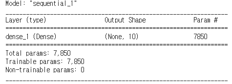
8. 모델 요약
총 10개의 로지스틱 회귀가 있고, 각 로지스틱 회귀는 784개의 회귀계수(W)와 1개의 편향(bias)를 갖고 있기 때문에 총 7850(785*10)개의 param이 있는 것을 확인할 수 있다.
model.summary()[출력]
model.layers[0].weights[출력]
[<tf.Variable 'dense_1/kernel:0' shape=(784, 10) dtype=float32, numpy=
array([[ 0.04938879, -0.07676695, -0.03612473, ..., -0.08555932,
-0.0155737 , 0.07637201],
[-0.0232266 , 0.02347476, 0.06019563, ..., -0.02940473,
0.06281503, 0.07443405],
[ 0.04140536, 0.07258698, -0.03491154, ..., -0.01304246,
0.07327399, 0.00835124],
...,
[ 0.04623742, 0.05178858, -0.01503239, ..., 0.00743634,
0.0776026 , -0.08589918],
[ 0.03308423, -0.04045485, -0.04682832, ..., -0.06863538,
-0.00120455, -0.03433972],
[ 0.08357991, -0.0211922 , 0.05378201, ..., 0.04312288,
0.00650842, 0.0051019 ]], dtype=float32)>,
<tf.Variable 'dense_1/bias:0' shape=(10,) dtype=float32, numpy=
array([-0.07876502, 0.16116439, -0.03372397, -0.06804138, 0.05435583,
0.15498637, -0.00570482, 0.09562831, -0.2344925 , -0.04540703],
dtype=float32)>]
'Machine Learning > Coding' 카테고리의 다른 글
| [실습]주성분 분석(Principal Component Analysis, PCA) (0) | 2021.07.13 |
|---|---|
| [실습] Linear Regression(선형회귀) (0) | 2021.06.27 |
| [실습] KMeans (K 평균 군집화) (0) | 2021.06.23 |
| [실습] 랜덤 포레스트(Random Forest)와 앙상블(Ensemble) (0) | 2021.06.20 |
| [실습] 다항분포 나이브 베이즈(Multinomial Naive Bayes) (0) | 2021.06.13 |