2. Theoretical formulations
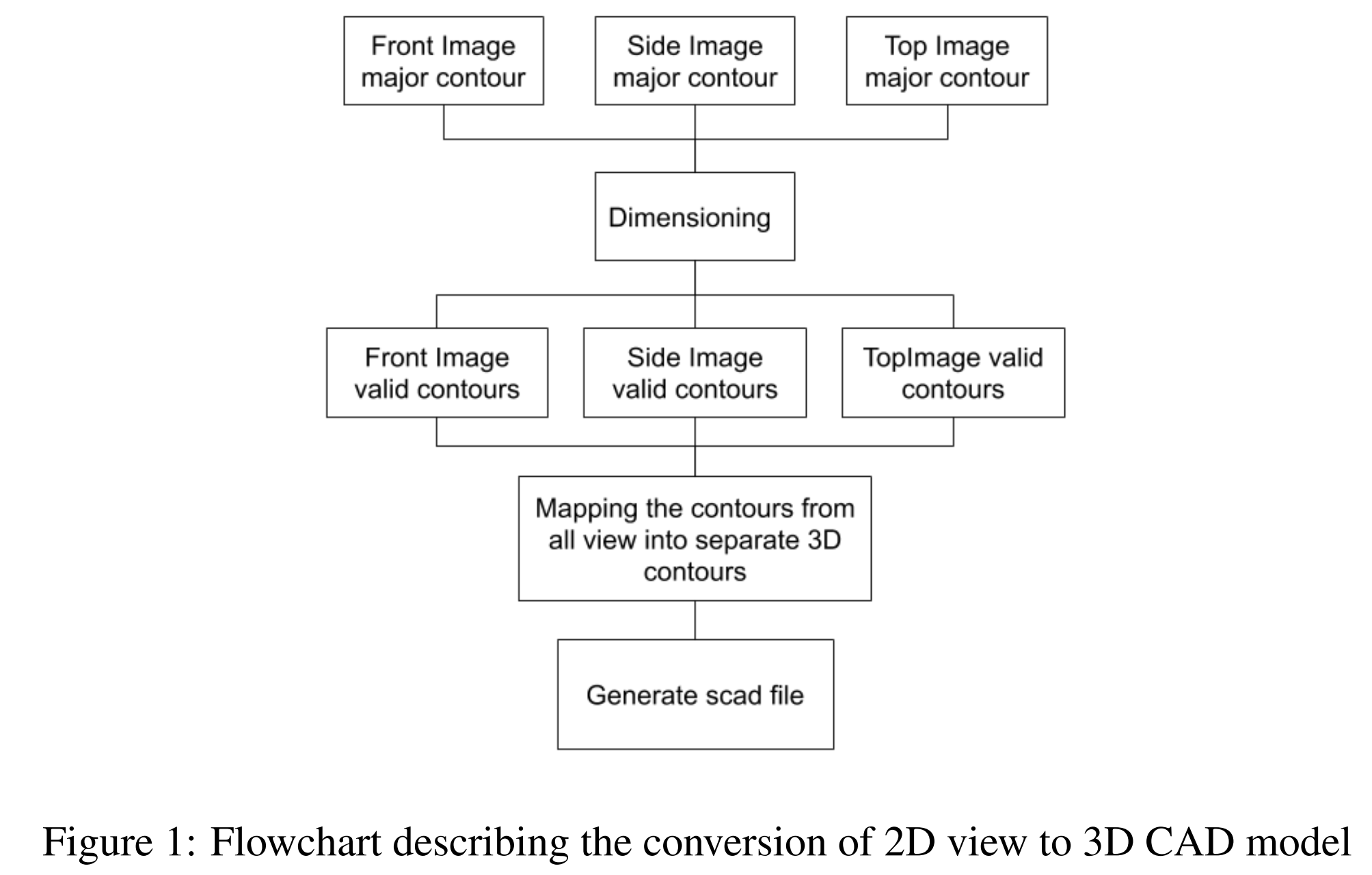
2D drawing 사본 또는 drawing 사진으로 시작한다. (사본, 사진으로 실험을 했다는 내용같음) 가장 중요한 이론의 아이디어는 현재 섹션에서는 생략한다. 전체 flow는 Figure 1을 확인하면 된다.
re-construction 프로세스와 관련된 단계는 다음과 같다.
- outer boundary를 detection하고 bounding box를 development
- bounding box를 참조하여 point 위치를 결정
- 모든 points of interest 를 SCAD 포맷의 3D CAD 모델로 최종 변환
2.1. Contour detection
첫 번째 단계는 이미지를 feature가 식별될 수 있는 form으로 변환하는 것과 관련이 있다.
edge, contour는 일반적으로 서로 혼용(?)될 수 있지만 컴퓨터 그래픽에서는 다른 것을 의미한다. (보통 edge가 contour가 될 수 있고 contour는 edge가 될 수 있는데 컴퓨터 그래픽에서는 다르다는 말 같다.) edge는 인접한 point와 비교하여 값이 크게 변경되는 point이다. (값이 크게 바뀐다는 말이 이해가 안간다.) 그래서 edge의 개념은 로컬 범위 안에 있다(???)
반면에 contour는 어떤 모양의 boundary를 묘사하고 edge가 포함된 닫힌 곡선이다. countour line은 같은 값 또는 같은 강도(진한 정도?)의 boundary로 표현된 곡선을 가르킨다. 그래서 contour line은 전체적인 모양의 boundary에 있다. (edge의 개념이 로컬 범위에 있고 countour는 전체적인 모양의 boundary에 있다는 말을 쉽게 말하면 edge가 contour에 속한다라고 말할 수 있을 것 같다.)
OpenCV를 사용하여 계산된 contours는 contour line들을 구성하는 point들의 list이고 contours를 면적으로 정렬하여 2D drawing의 외곽선을 그려야한다.
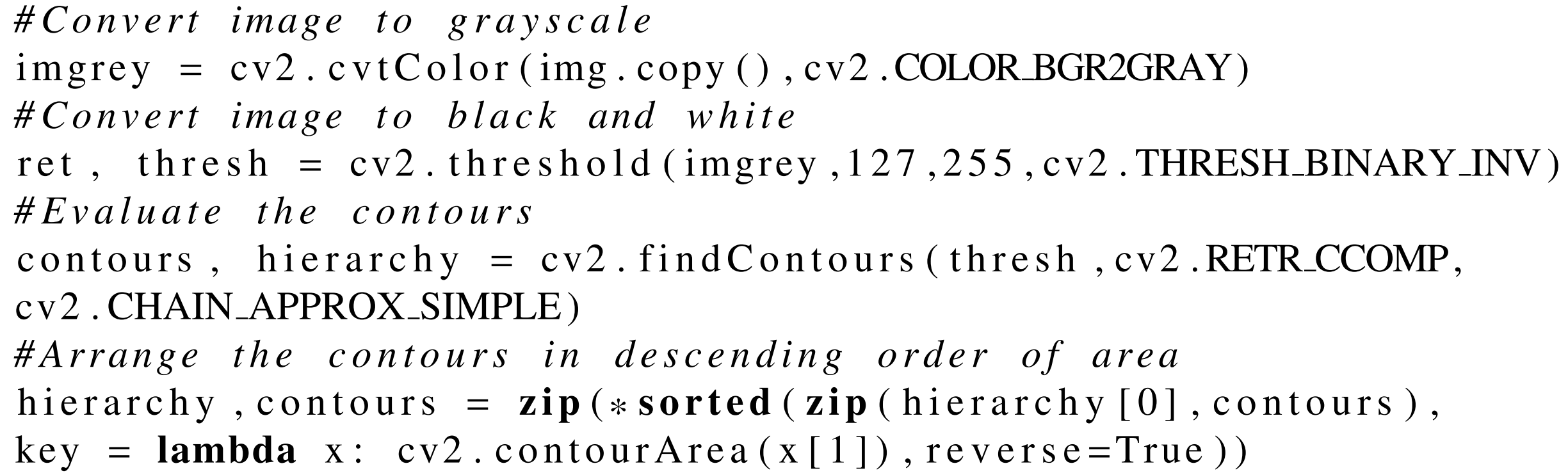
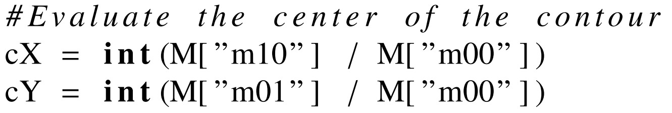
이미지에서 feature를 추출하기위해서 bounding box가 필요하다. 그래서 contour의 극좌표와 center 좌표를 찾아낼 필요가 있다. 위에서 수행했던 것처럼 이미지를 grayscale하고 contours를 추출하면 Opencv function cv2.moments()로 contour에 대해 계산된 모든 moment 값들의 dictionary를 추출할 수 있다.
mechanic에서 moment는 힘과 거리의 곱으로 표현한다. computer vision에서 이것은 이미지의 중심으로 표현하고 픽셀 강도(값)의 weighted average로 표현된다. 수식으로는 다음과 같이 표현된다.
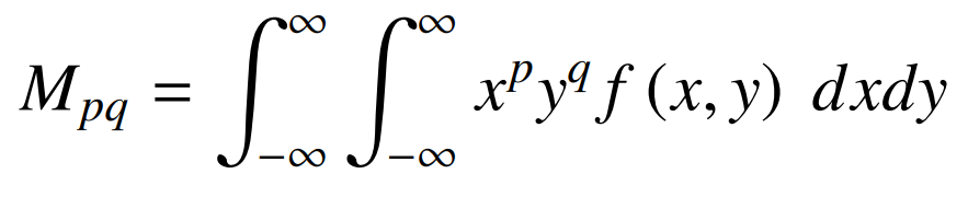
p, q = 0, 1, 2, ...
이것은 raw image의 moments $M_{ij}$를 찾아내기위해 픽셀 강도 $I(x,y)$를 가지는 grayscale image에 적용될 수 있다.
이미지의 중심은 다음과 같이 주어진다.
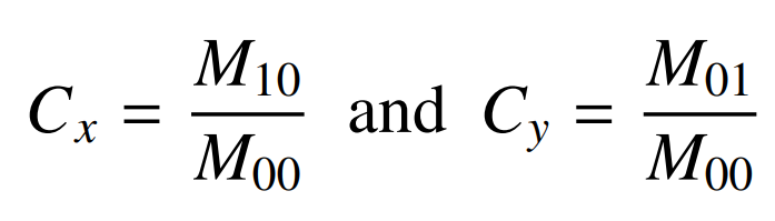
모양의 끝 부분을 찾아내기위한 마지막 단계 중 하나로 bounding box evaluation을 포함한다. Figure 2를 보는 것처럼 object of interest는 rotate될 수 있다. 그래서 bounding rectangle의 최소 면적을 분석하기위해 객체의 rotation과 극좌표 모두 고려할 필요가 있다.
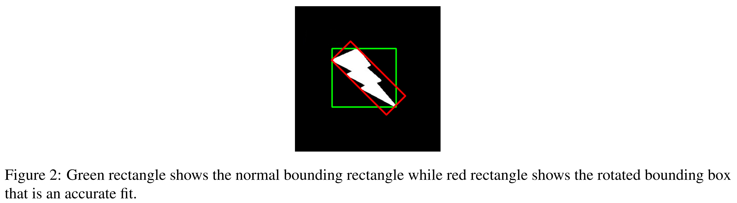
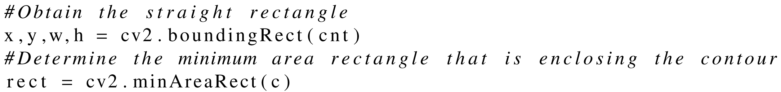
위 코드에서 cnt는 contours 중 하나이고 c도 마찬가지 인 것 같다. 단지 변수를 구분해준 것 같다. (cnt = c) 코드와 Figure2를 비교해서 본다면 cv2.boundingRect는 초록색 박스이고 cv2.minAreaRect는 빨간색 박스이다.
2.2. Point location
어떤 point가 주어지면 특정 contour의 바깥쪽에 있는지 안쪽에 있는지 알아낼 필요가 있다. signed distance function은 contour와 관련된 점의 위치를 알아내기위해 사용될 수 있다. 이 함수의 return 값 +1 / -1 / 0은 각각 contour의 안쪽 / 바깥쪽 / contour 선 상에 있다는 것을 의미한다.

2.3. Conversion to 3D model
마지막 단계는 3D solid로 변환하는데 필요한 2D shape 인식과 관련이 있다. 여기서 여섯 가지의 shape(삼각형, 정사각형, 직사각형, 오각형, 육각형, 원)을 고려한다. Ramer–Douglas–Peucker 알고리즘은 곡선을 point set으로 변환하기위해 사용된다.
# 본 논문에 작성된 코드를 약간 수정한 부분이 있다.
def detect(c):
    # Initialize the shape name and approximate the contour
    shape = "unidentified"
    peri = cv2.arcLength(c, True)
    # Finding the number of line segment required to make the polygon
    approx = cv2.approxPolyDP(c, 0.015 * peri, True)
    # Cylinder type in openscad for making regular prism
    cylinder_type = 0

    # If the shape is a triangle, it will have 3 vertices
    if len(approx) == 3:
        shape = "triangle"
        cylinder_type = 3

    # If the shape had 4 vertices, it is either a square or a rectangle
    elif len(approx) == 4:
        # compute the bounding box of the contour and use the
        # bounding box to compute the aspect ratio
        rect = cv2.minAreaRect(c)
        ar = rect[1][0] / float(rect[1][1])
        # a square will have an aspect ratio that is approximately
        # equal to one, otherwise, the shape is a rectangle
        shape = "square" if 0.999 <= ar <= 1.001 else " rectangle"

   # If the shape is a pentagon, it will have 5 vertices
   elif len(approx) == 5:
       shape = "pentagon"
       cylinder_type = 5

   # If the shape is a hexagon, it will have 6 vertices
   elif len(approx) == 6:
       shape = "hexagon"
       cylinder_type = 6

   # otherwise, we assume the shape is a circle
   else:
       shape = "circle"
       cylinder_type = 1

   # return the name of the shape
   return shape, cylinder_type
마지막으로 분석된 shape은 SCAD 포맷의 3D solid로 다음과 같이 주어져 변환된다.
- sphere(r=radius)
- cube(size=[x,y,z], center=true/false) -> 여기서 중심은 (0, 0)
- cylinder(h, r1, r2, center, fn : fixed number of fragments)
또한 다음과 같이 union(), difference()로 더 복잡한 shape, object를 만들어낼 수 있다.
